 Stewy Slocum
Hutchinson's Diagonal Estimator
In this post, we’ll take a look at a method of approximating large Hessian matrices using a stochastic diagonal estimator. Hutchinson’s method can be used for optimization and loss-landscape analysis in deep neural networks.
In modern machine learning with large deep models, explicit computation of the Hessian matrix is intractable. However, the Hessian matrix provides valuable information for optimization, studying generalization, and for other purposes. But even if we can’t calculate the full Hessian, can we effectively approximate it?
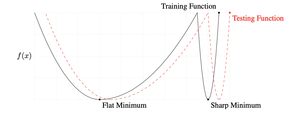 Fig. 1. Flat minima have been linked to improved generalization. The magnitude of the eigenvalues of the Hessian provide one way to characterize sharpness/flatness (Keskar et al., 2017).
There has been significant work towards efficient approximation of the Hessian, most notably in the form of low-rank updates like L-BFGS. This approach work well in traditional optimization settings, but is relatively slow and generally doesn’t work in stochastic settings (Bollapragada et al., 2018).
Alternatively, there has also been a variety of work old and new to estimate the diagonal of the Hessian as a way of approximating the matrix as a whole, for pruning (LeCun et al., 1989), (Hassibi & Stork, 1992) analyzing the loss landscape (Yao et al., 2020), and optimization (Yao et al., 2021). It has been argued that the diagonal is a good approximation to the Hessian for machine learning problems, and that diagonal elements tend to be much larger than off-diagonal elements.
However, calculating the diagonal of the Hessian is not straightforward. Automatic differentiation libraries are designed to make large computations in parallel, so naively calculating diagonal terms of the Hessian one-by-one \(\frac{\partial^2 L(x)}{\partial x_1^2}, \frac{\partial^2 L(x)}{\partial x_2^2}, ..., \frac{\partial^2 L(x)}{\partial x_n^2}\) requires \(n\) backprop operations and isn’t computationally feasible. However, we can estimate this diagonal relatively efficiently using randomized linear algebra in the form of Hutchinson’s estimator.
Hessian-Vector Products
While calculating the Hessian as a whole isn’t possible, we can efficiently estimate Hessian-vector products. There are a variety of ways to do this, the simplest being a finite difference approximation:
1. Finite Difference Approximation
\[H(x) v \approx \frac{g(x + rv) - g(x - rv)}{2r}\]The error of this approximation is \(O(r)\), which means it can be quite accurate when \(r\) is small. However, as \(r\) becomes small, rounding errors pile up in the numerator. While not accurate enough for every application, the finite difference approximation is simple and cheap (2 gradient evaluations).
2. Product Rule Trick
\[\frac{\partial (g(x)^\top v)}{\partial x} = \frac{\partial g(x)}{\partial x} v + g(x) \frac{\partial v}{\partial x} = \frac{\partial g(x)}{\partial x} v = H(x) v\]This exact method requires taking the gradient of an expression that includes the gradient. It means that the operations used to backprop must also be tracked so they can be differentiated. This method is also \(O(n)\) like typical gradient evaluations, but because of the more complex underlying expression, the constant factors are slightly higher in memory and in time. The product rule trick is the implementation you’ll find for Hessian-vector products in pytorch and jax.
Hutchinson’s Estimator
Now that we have efficient Hessian-vector multiplication, we can use Hutchinson’s estimator.
Hutchinson’s Trace Estimator
Hutchinson’s original estimator is for the trace of a matrix. This estimator is more common than the diagonal estimator and has been more thoroughly analyzed, so let’s warm up by taking a look at it.
To estimate the trace, we draw random vectors \(z\) from a distribution with mean zero and variance one (typically the Rademacher distribution). We can then estimate the trace of a matrix as \(\mathbb{E}[z^\top H z] = \text{trace}(H)\).
Theorem: Let \(z\) a random vector with \(\mathbb{E}[z]=0\), \(\mathbb{V}[z]=1\), and independent entries. Then \(\mathbb{E}[z^\top H z] = \text{trace}(H)\).
Proof.
\[\begin{align} \mathbb{E}[z^\top H z] &= \mathbb{E}[\begin{bmatrix}z_1 \\ z_2 \\ ... \\ z_n\end{bmatrix}^\top \begin{bmatrix}H_{11} z_1 + H_{12} z_2 + ... + H_{1n} z_n \\ H_{12} z_1 + H_{22} z_2 + ... + H_{2n} z_n \\ ... \\ H_{n1} z_1 + H_{n2} z_2 + ... + H_{nn} z_n\end{bmatrix}] \\ &= \mathbb{E}[\begin{bmatrix}z_1 \\ z_2 \\ ... \\ z_n\end{bmatrix}^\top \begin{bmatrix}\sum\limits_{i=1}^n H_{1i} z_i \\ \sum\limits_{i=1}^n H_{2i} z_i \\ ... \\ \sum\limits_{i=1}^n H_{ni} z_i\end{bmatrix}] \\ &= \mathbb{E}[z_1 \sum\limits_{i=1}^n H_{1i} z_i + z_2 \sum\limits_{i=1}^n H_{2i} z_i + ... + z_n \sum\limits_{i=0}^n H_{ni} z_i] \\ &= \sum\limits_{i=1}^n H_{1i} \mathbb{E}[z_1 z_i] + \sum\limits_{i=1}^n H_{2i} \mathbb{E}[z_2 z_i] + ... + \sum\limits_{i=1}^n H_{ni} \mathbb{E}[z_n z_i] \\ \end{align}\]And since the entries of \(z\) are independent, \(\mathbb{E}[z_i z_j] = \mathbb{E}[z_i]\mathbb{E}[z_j] = 0 \cdot 0 = 0\) for \(i \neq j\).
However, when \(i = j\), then \(\mathbb{E}[z_i z_j] = \mathbb{E}[z_i^2] = \mathbb{V}[z_i] + \mathbb{E}[z_i]^2 = 1 + 0^2 = 1\).
So
\[\begin{align} \mathbb{E}[z^\top H z] &= \sum\limits_{i=1}^n H_{1i} \mathbb{E}[z_1 z_i] + \sum\limits_{i=1}^n H_{2i} \mathbb{E}[z_2 z_i] + ... + \sum\limits_{i=1}^n H_{ni} \mathbb{E}[z_n z_i] \\ &= H_{11} + H_{22} + ... + H_{nn} \\ &= \text{trace}(H) \tag*{$\blacksquare$} \end{align}\]Hutchinson’s Diagonal Estimator
The basic idea from the trace estimator can be modified to give an estimator for the diagonal rather than the trace.
Theorem: Let \(z\) be a random variable \(z\) with \(\mathbb{E}[z]=0\), \(\mathbb{V}[z]=1\), and independent entries. Then \(\mathbb{E}[z \odot H z] = \text{diag}(H)\).
Proof.
\[\begin{align*} \mathbb{E}[z \odot Hz] &= \mathbb{E}[ \begin{bmatrix}z_1 \\ z_2 \\ ... \\ z_n\end{bmatrix} \odot \begin{bmatrix} H_{11} z_1 + H_{12} z_2 + ... + H_{1n} z_n \\ H_{21} z_1 + H_{22} z_2 + ... + H_{2n} z_n \\ ... \\ H_{n1} z_1 + H_{n2} z_2 + ... + H_{nn} z_n \end{bmatrix} ] \\ &= \begin{bmatrix} H_{11} \mathbb{E}[z_1^2] + H_{12} \mathbb{E}[z_1z_2] + ... + H_{1n}[z_1z_n] \\ H_{21} \mathbb{E}[z_2z_1] + H_{22} \mathbb{E}[z_2^2] + ... + H_{2n}[z_2z_n] \\ ... \\ H_{n1} \mathbb{E}[z_nz_1] + H_{n2} \mathbb{E}[z_nz_2] + ... + H_{nn}[z_n^2] \end{bmatrix} \\ &= \begin{bmatrix} H_{11} \\ H_{22} \\ ... \\ H_{nn} \end{bmatrix} \\ &= \text{diag}(H) \tag*{$\blacksquare$} \end{align*}\]Now let’s calculate the variance of Hutchinson’s diagonal estimator.
Theorem: Let \(z \sim \text{Rademacher}\). Then the covariance matrix of Hutchinson’s diagonal estimator is
\[\begin{align} \Sigma_{z \odot Hz} = \text{diag}(H)\text{diag}(H)^\top + \left(\begin{bmatrix} ||H_1||^2 \\ ||H_2||^2 \\ \vdots \\ ||H_n||^2 \end{bmatrix} - 2 \text{diag}(H)^2\right) \odot I \end{align}\]where \(H_i\) is the \(i\)-th row of \(H\).
Proof. Let us consider each entry of the covariance matrix separately:
\[\begin{align} (\Sigma_{z \odot Hz})_{ij} &= \text{Cov}[(z \odot Hz)_i (z \odot Hz)_j] \\ &= \mathbb{E}[(z \odot Hz)_i (z \odot Hz)_j] - \mathbb{E}[z \odot Hz]_i \mathbb{E}[z \odot Hz]_j \\ &= \mathbb{E}[(z_i (H_{i1} z_1 + ... + H_{in} z_n)) (z_j (H_{j1} z_1 + ... + H_{jn} z_n))] - H_{ii} H_{jj} \\ &= \mathbb{E}[\sum\limits_{k=0}^n \sum\limits_{l=0}^n H_{ik}H_{jl} z_i z_k z_j z_l] - H_{ii}H_{jj} \\ &= (\sum\limits_{k=0}^n \sum\limits_{l=0}^n H_{ik} H_{jl} \mathbb{E}[z_i z_k z_j z_l]) - H_{ii}H_{jj} \end{align}\]First consider diagonal elements, which have \(i = j\):
- Case 1. \(i = j = k = l\). Then \(\mathbb{E}[z_i z_k z_j z_l] = \mathbb{E}[z_i^4] = \text{Kurtosis}[z]\)
- Case 2. \(i = j \neq k\), \(k = l\). Then \(\mathbb{E}[z_i z_k z_j z_l] = \mathbb{E}[z_i^2]\mathbb{E}[z_k^2] = 1 \cdot 1 = 1\)
- Case 3. \(i = j\), \(k \neq l\). Therefore, at least one of \(k, l \neq i\). WLOG suppose \(k \neq i\). Then \(\mathbb{E}[z_i z_k z_j z_l] = \mathbb{E}[z_i^2 z_l]\mathbb{E}[z_k] = 0 \cdot \mathbb{E}[z_i^2 z_l] = 0\)
This gives
\[\begin{align} (\Sigma_{z \odot Hz})_{ii} &= (\sum\limits_{k=0}^n \sum\limits_{l=0}^n H_{ik} H_{il} \mathbb{E}[z_i z_k z_i z_l]) - H_{ii}^2 \\ &= \text{Kurtosis}[z]H_{ii}^2 + \sum\limits_{k=0, k \neq i}^n H_{ik}^2 - H_{ii}^2 \\ &= \sum\limits_{k=0, k \neq i}^n H_{ik}^2 \end{align}\]since the kurtosis of a Rademacher RV is 1. In fact, the Bernoulli distribution has the smallest kurtosis of any distribution at 1, and since the Rademacher distribution is just a scaled Bernoulli, it is the optimal distribution to draw \(z\) from with respect to the variance of our estimator.
Now consider off-diagonal elements, which have \(i \neq j\):
- Case 1. \(i \neq j\) with \(i = k, j = l\) or \(i = l, j = k\). Then \(\mathbb{E}[z_i z_k z_j z_l] = \mathbb{E}[z_i^2]\mathbb{E}[z_j]^2 = 1 \cdot 1 = 1\)
- Case 2. \(i \neq j\) with at least one of \(k, l\) not equal to \(i\) or \(j\). WLOG suppose \(k \neq i, j\). Then \(\mathbb{E}[z_i z_k z_j z_l] = \mathbb{E}[z_i z_j z_l]\mathbb{E}[z_k] = \mathbb{E}[z_i z_j z_l] \cdot 0 = 0\)
This gives
\[\begin{align} (\Sigma_{z \odot Hz})_{ij} &= (\sum\limits_{k=0}^n \sum\limits_{l=0}^n H_{ik} H_{jl} \mathbb{E}[z_i z_k z_j z_l]) - H_{ii}H_{jj} \\ &= 2H_{ii}H_{jj} - H_{ii}H_{jj} \\ &= H_{ii}H_{jj} \end{align}\]So our final covariance matrix is
\[\require{color} \definecolor{brand}{RGB}{78, 182, 133} \begin{align} \Sigma_{z \odot Hz} &= \begin{bmatrix} \textcolor{brand}{\sum\limits_{k=0, k \neq 1}^n H_{1k}^2} & H_{11}H_{22} & H_{11}H_{33} & ... & H_{11}H_{nn} \\ H_{11}H_{22} & \textcolor{brand}{\sum\limits_{k=0, k \neq 2}^n H_{2k}^2} & H_{22}H_{33} & ... & H_{22}H_{nn} \\ H_{11}H_{33} & H_{22}H_{33} & \textcolor{brand}{\sum\limits_{k=0, k \neq 3}^n H_{3k}^2} & ... & H_{33}H_{nn} \\ \vdots & \vdots & \vdots & \ddots & H_{n-1n-1}H_{nn} \\ H_{11}H_{nn} & H_{22}H_{nn} & H_{33}H_{nn} & ... & \textcolor{brand}{\sum\limits_{k=0, k \neq n}^n H_{nk}^2} \end{bmatrix} \\ &= \underbrace{\text{diag}(H)\text{diag}(H)^\top - \text{diag}(H)^2 \odot I}_{\text{off-diagonal covariances}} + \underbrace{\textcolor{brand}{\left(\begin{bmatrix} ||H_1||^2 \\ ||H_2||^2 \\ \vdots \\ ||H_n||^2 \end{bmatrix} - \text{diag}(H)^2\right) \odot I}}_{\text{diagonal vector of variances}} \\ &= \text{diag}(H)\text{diag}(H)^\top + \left(\begin{bmatrix} ||H_1||^2 \\ ||H_2||^2 \\ \vdots \\ ||H_n||^2 \end{bmatrix} - 2 \text{diag}(H)^2\right) \odot I \tag*{$\blacksquare$} \end{align}\]Note that variance of our estimator (diagonal of tbe covariance matrix) at a specific output \(i\) is \(\mathbb{V}[(z \odot H z)_i] = \textcolor{brand}{\sum\limits_{k=0, k \neq i}^n H_{ik}^2} = \| H_i \| ^2 - H_{ii}^2\). Interestingly, this variance is equal to the squared L-2 norm of the off-diagonal elements of each row. So even though this variance grows like \(O(n)\) with the number of variables in the Hessian, if the assumption that the off-diagonal elements of the Hessian are small is true, then this variance remains small.
Now let’s take a break with this landscape by Rembrandt

The Mill
Courtesy National Gallery of Art, Washington
References
- Keskar, N., Mudigere, D., Nocedal, J., Smelyanskiy, M., & Tang, P. T. P. (2017). On Large-Batch Training for Deep Learning: Generalization Gap and Sharp Minima. ArXiv, abs/1609.04836.
- Bollapragada, R., Nocedal, J., Mudigere, D., Shi, H.-J., & Tang, P. T. P. (2018). A progressive batching L-BFGS method for machine learning. International Conference on Machine Learning, 620–629. https://arxiv.org/abs/1802.05374
- LeCun, Y., Denker, J., & Solla, S. (1989). Optimal Brain Damage. NIPS.
- Hassibi, B., & Stork, D. (1992). Second Order Derivatives for Network Pruning: Optimal Brain Surgeon. NIPS.
- Yao, Z., Gholami, A., Keutzer, K., & Mahoney, M. W. (2020). PyHessian: Neural Networks Through the Lens of the Hessian. 2020 IEEE International Conference on Big Data (Big Data), 581–590.
- Yao, Z., Gholami, A., Shen, S., Keutzer, K., & Mahoney, M. (2021). ADAHESSIAN: An Adaptive Second Order Optimizer for Machine Learning. ArXiv, abs/2006.00719.